In this assignment, you will implement mass spring, linear FEM and corotational FEM deformable object simulators to deform a 2D object. The 2D object is represented as an obj mesh. Our starter code can load the mesh, and render the mesh. Our starter code also implements a GUI for user interaction. Your task is to fill in the missing functions and code blocks in the starter code.
You can download the starter code and data here.
For Mac and Linux users, please enter the "imgui" folder and run
$maketo compile the code.
$brew install freeglut(Note that although macOS comes with a GLUT framework, it is now deprecated and may not be stable.) Then, open Makefile, replace the correct freeglut version number in the line:
OPENGL_LIBS=-framework OpenGL /usr/local/Cellar/freeglut/3.2.1/lib/libglut.dylibNow you should be able to compile the starter code in macOS.
The driver needs a single argument to run. The argument is the filename of the configuration file. For example: <starter code folder>/examples/square/run.config. For Windows users, this argument has been added to the project properties. Launch the driver using the debug button in VS2017 and the correct configuration will be loaded. For macOS and Linux users, execute <starter code folder>/run.sh to launch the driver with the proper configuration file. After launching the driver, the 2D mesh is rendered using OpenGL. Further instructions:
Important: When you compile the starter code, you will see the 2D mesh rendered. However, there will be no deformation even if you enable gravity or drag a vertex on the mesh. After you implement the required code blocks, the mesh should deform under external forces, while the fixed vertices are fixed to its rest positions.
Please remember that all vertices are in 2D in this assignment. For example, a vertex's position is \(p_A=(p_A^x, p_A^y)\). Its displacement is \(u_A=(u_A^x,u_A^y)\).
For a physics-based simulation system, it is important to calculate the mass matrix for the simulated object. For the mass spring system, the object is represented by vertices connected by springs. In FEM, the object is represented by a set of elements which is triangles in our 2D case in this homework, or tetrahedra in 3D case. No matter how we express the objects, calculation of mass follows the formula \[m_e = \rho * V(e).\] Here, \(V(e)\) is the volume of a 3D element or the surface area of a 2D element and \(\rho\) is the mass density. In order to build the mass matrix \(M\in R^{2n*2n}\) for our system, we need to first calculate mass for each vertex. We iterate each triangle to get the surface area \(V(e)\) for each triangle. Then we compute \(m_e = \rho * V(e)\) for each triangle. Next we allocate the mass value to three vertices on the triangle, that is to say, each vertex represents a third of the element mass. Suppose the three vertices on the triangle are \(A,B,C\), then we have \[m_A = \dfrac{1}{3} m_e \] \[m_B = \dfrac{1}{3} m_e \] \[m_C = \dfrac{1}{3} m_e \] Under these assumptions, \(M\) is a diagonal matrix; this is called "mass lumping". Students are required to implement the calculation of the mass for each vertex in baseModel2D.cpp.
Assume A and B are two mass points connected with a spring. Let \(\vec{L}\) be the vector pointing from B to A, \(\vec{L}=p_A-p_B\). Let \(R\) be the spring rest length. Then the elastic force exerted on A is: \[\vec{f}_A = -k_{hook}(|\vec{L}|-R)\dfrac{\vec{L}}{|\vec{L}|},\] where \(k_{hook}\) is the hook stiffness value. According to Newton's 3rd law: if object A exerts a force \(f\) on object B, then object B is at the same time exerting force \(-f\) on A. So the elastic force exerted on particle B is \(-\vec{f}_A\). The elastic energy stored in the spring is therefore \[E_{elastic} = \dfrac{1}{2}k_{hook}(|\vec{L}|-R)*(|\vec{L}|-R).\] Stiffness matrix is also sometimes needed in simulation system. The stiffness matrix is the gradient of the internal force with respect to the displacements. For a spring, the stiffness matrix \(K_e\in R^{4*4}\) is calculated as follows \[K_e =\dfrac{\partial [\begin{matrix}\vec{f}_A\\\vec{f}_B\end{matrix}]}{\partial [\begin{matrix}u_A\\u_B\end{matrix}]} = [\begin{matrix}\dfrac{\partial \vec{f}_A}{\partial u_A} & \dfrac{\partial \vec{f}_A}{\partial u_B}\\\dfrac{\partial \vec{f}_B}{\partial u_A} & \dfrac{\partial \vec{f}_B}{\partial u_B} \end{matrix}] = [\begin{matrix}K_{AA} & -K_{AA}\\-K_{AA} & K_{AA}\end{matrix}],\] where \(K_{AA}\in R^{2*2}\) is the gradient of the internal force on particle A with respect to \(u_A\). In order to calculate \(K_{AA}\), we can use the following formula \[K_{AA} = \dfrac{\partial \vec{f}_A}{\partial u_A} = k_{hook}(I^{2*2}-R[\begin{matrix} \dfrac{1}{L} - \dfrac{1}{L^3}(p_A^x-p_B^x)*(p_A^x-p_B^x) & -\dfrac{1}{L^3}(p_A^x-p_B^x)*(p_A^y-p_B^y) \\ -\dfrac{1}{L^3}(p_A^x-p_B^x)*(p_A^y-p_B^y) & \dfrac{1}{L} - \dfrac{1}{L^3}(p_A^y-p_B^y)*(p_A^y-p_B^y) \end{matrix}])\] Students are required to implement calculation of elastic energy, internal forces and stiffness matrix for each element (spring) in massSpring2D.cpp.
In linear FEM, we assume a linear relationship between the internal force and displacements, which is, \[\vec{f} = K * \vec{u},\] where \(K\in R^{2n*2n}\) is the stiffness matrix of the system and \(\vec{u}\in R^{2n*1}\) is the displacements. And the elastic energy is therefore, \[E_{elastic} = \dfrac{1}{2}\vec{u}^T * K * \vec{u}.\] In linearFEM2D.cpp, we provided the precomputed stiffness matrix for each element (triangle). Students are required to fill in the stiffness matrix and implement calculation of the elastic energy and internal force for each element. For more details on how to calculate the stiffness matrix, please refer to [Muller 04].
The shortcoming of the linear FEM is that is not rotation-invariant. This leads to obvious artifacts under large deformations. Corotational linear FEM addresses this by extracting the rotational component of the deformation gradient. It then computes the internal forces. The rotations are extracted separately for each element (triangle). Suppose the three triangle vertices are \(A,B,C\). Let \(p_{A,B,C}\) represent the deformed vertex positions, whereas \(q_{A,B,C}\) represents the undeformed vertex positions. We define the deformation mapping function \(\phi\) that maps the undeformed positions of the element to its deformed positions. We also define the deformation gradient matrix \(F\in R^{2*2}\) as the Jacobian matrix of \(\phi\). Each vertex satisfies the following mapping formulas, \[\vec{p}_A = \phi(\vec{q}_A) = F_e \vec{q}_A + t_e,\] \[\vec{p}_B = \phi(\vec{q}_B) = F_e \vec{q}_B + t_e,\] \[\vec{p}_C = \phi(\vec{q}_C) = F_e \vec{q}_C + t_e.\] Here, \(F_e\) contains the rotational and stretching parts of the element deformation and \(t_e\) contains the translation part. To eliminate \(t_e\) in the formula, we subtract the last equation from the other two. We then group the two resulted equations into a single matrix equation as follows, \[[\begin{matrix} \vec{p}_A^x - \vec{p}_C^x & \vec{p}_B^x - \vec{p}_C^x \\ \vec{p}_A^y - \vec{p}_C^y & \vec{p}_B^y - \vec{p}_C^y \end{matrix}] = F_e * [\begin{matrix} \vec{q}_A^x - \vec{q}_C^x & \vec{q}_B^x - \vec{q}_C^x \\ \vec{q}_A^y - \vec{q}_C^y & \vec{q}_B^y - \vec{q}_C^y \end{matrix}] \Rightarrow D_e^s = F_e * D_e^m .\] It is easy to calculate \(D_e^s\) and \(D_e^m\) for each element. Therefore, we calculate the deformation gradient as \(F_e = D_e^s * (D_e^m)^{-1}\). The rotational part \(R_e\) of the deformation gradient can be extracted by a Polar Decomposition of \(F_e\) as, \[F_e = R_e * S_e.\] Finally, we compute the internal forces as follows, \[\vec{f}_e = R_EK_e(R_E^{-1}\vec{p}_e - \vec{q}_e).\] Note that \(\vec{f}_e \in R^{6*1}, K_e \in R^{6*6}\). Matrix \(R_E \in R^{6*6}\) contains three copies of the \(2*2\) rotation matrix \(R_e\) along its diagonal. Vector \(\vec{p}_e \in R^{6*1}\) contains the deformed positions, whereas vector \(\vec{q}_e\in R^{6*1}\) contains the undeformed positions. The inverse rotation is \(R_e^{-1} = R_e^T\) since \(R_e * R_e^T = I\). The warped stiffness matrix is \[K_e' = R_EK_eR_E^{-1}.\] The elastic energy of the element is \[E_{elastic} = \dfrac{1}{2} (R_E^{-1}\vec{p}_e - \vec{q}_e)^T K_e (R_E^{-1}\vec{p}_e - \vec{q}_e).\] In corotationalLineaFEM2D.cpp, the precomputed unwarped stiffness matrix \(K_e\) is already provided. We also provide the function to do polar decomposition. Students are required to implement the internal froce, elastic energy and warped stiffness matrix calculation.
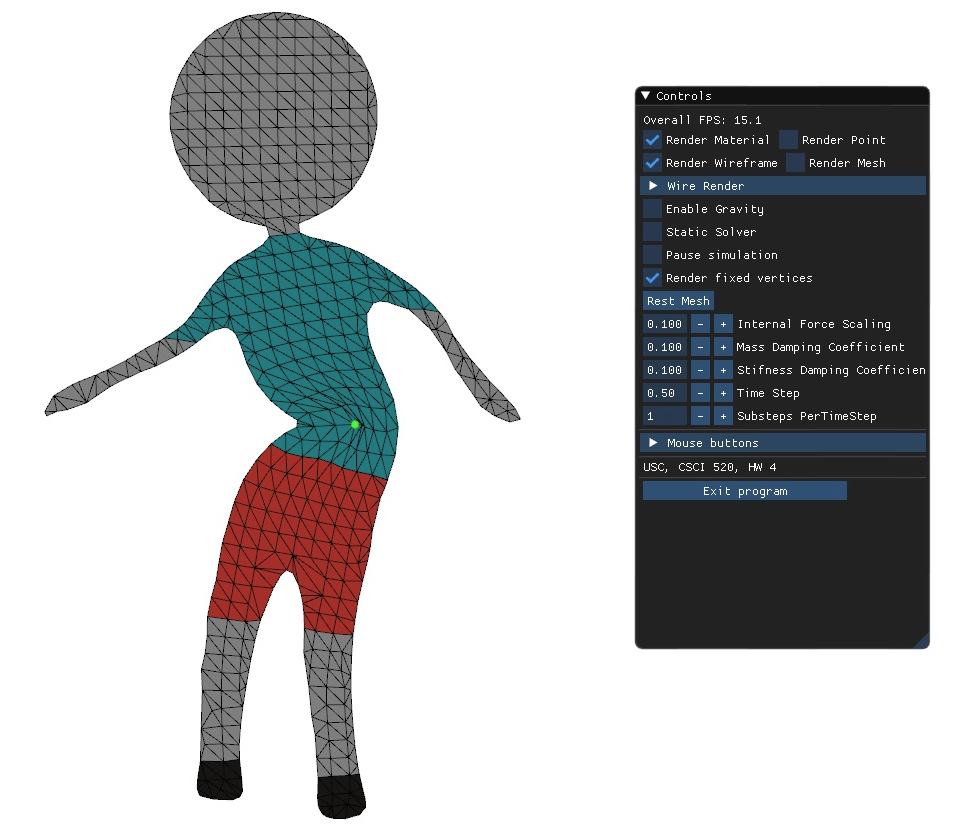
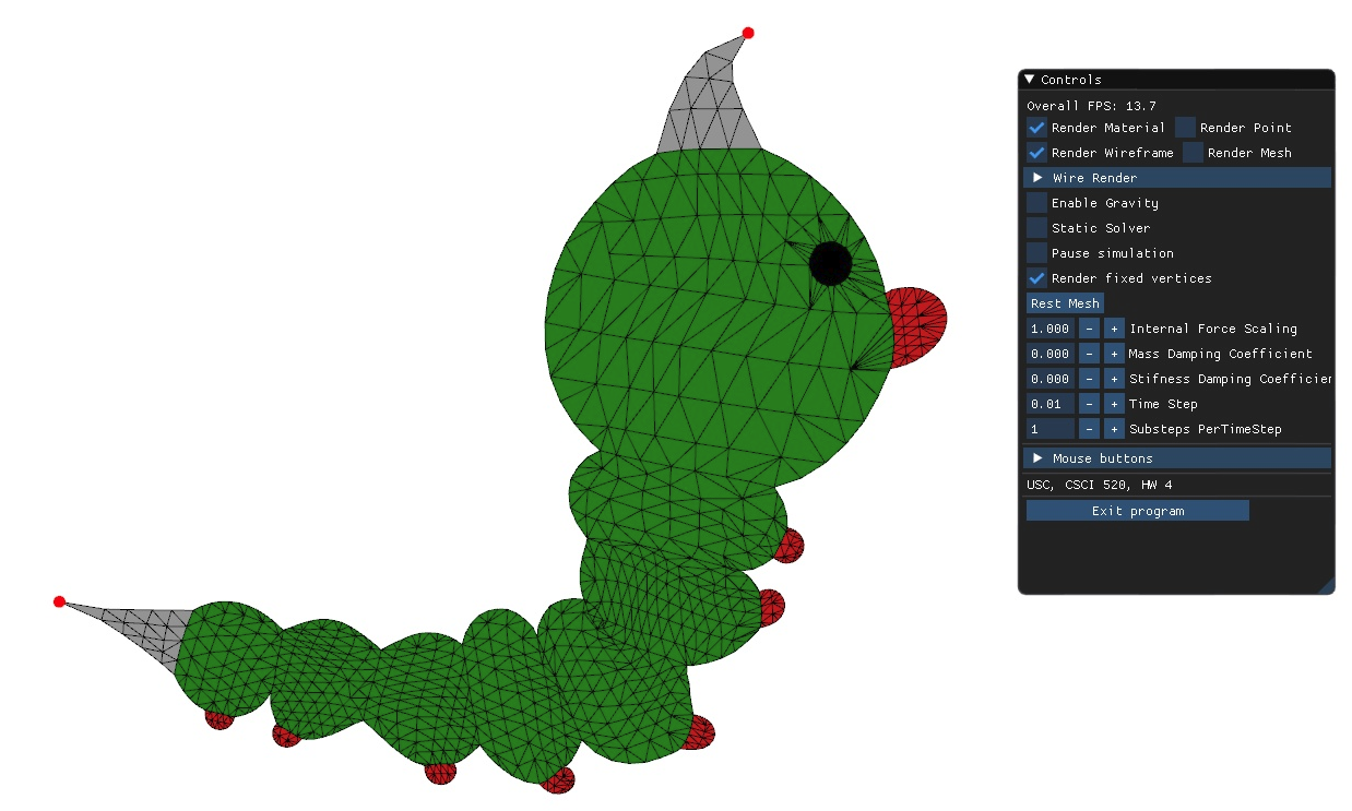
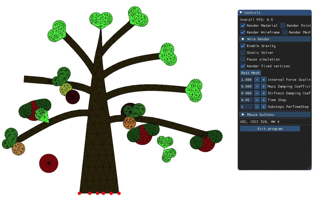
In the starter code, you will see several places marked with "Students should implement this." (or similar). These are the places where you need to provide your implementation. The assignment ships with four demos: square, fruit, weedle and stickman. You can switch between them by modifying run.sh.
Upload your entire solution as one zip file to the Blackboard. Your solution should include the following:
Please submit the assignment using the USC Blackboard. In order to do so, create a single zip file containing your entire submission. Submit this file to the blackboard using the "Attach File" field. After submission, please verify that your zip file has been successfully uploaded. You may submit as many times as you like. If you submit the assignment multiple times, we will grade your LAST submission only. Your submission time is the time of your LAST submission; if this time is after the deadline, late policy will apply to it.
Note: Blackboard has a limited upload bandwidth. To avoid uploading issues, please delete unnecessary files before submission. For example, Visual Studio will generate large redundant files. Remove them. Remove all object files (.obj, .o, or similar). Remove all intermediate compiling files (e.g. those in Debug/Release). Be careful to not accidentally erase your actual code files. Instructors and graders will read your code. Quality of your code and comments might affect your grade. This is an individual assignment. Your code might be compared to code of other students using (automatic) code comparison tools.
|
|
|
|